Waterman Polyhedra
 | Waterman Applet (below) doesn't work even though you installed Java? |
| Run the Waterman Web-Start Application instead. | |
| This downloads a jnlp (Java Web Start) file that tells Java how to run the Waterman outside of your browser. | |
| See my Java Web Start notes. |
Play with the controls! Use the "Sequence" slider to step through the series of polyhedra. Click the "Colors" button.
If you have red-blue 3D glasses, change the "Stereo Mode" to "Anaglyph".
If you have a ColorCode ViewerTM (see below), change the "Stereo Mode" to "ColorCode".
Further instructions are below the applet.
More Java applets here.
Contents:
- Browser/Java Notes
- Getting Started
- The Sequence Slider
- The Stereo Mode Choice
- The Color Scheme Choice
- The Orient Button
- Miscellaneous Notes
- What are Waterman Polyhedra?
- The Origin Choice
- Historical Notes
- Related Web Pages (links)
- Acknowledgements
- Version Notes
- Polyhedron Statistics
Browser/Java Notes:
- This is a Java 1.1 applet. See my Java page for Browser Requirements.
- Animations are disabled in browsers (like Netscape 4.7 for Windows) that don't honor my request to change "thread" priority.
- It's important to have the Java "Just In Time Compiler" enabled on your browser because this applet needs all the speed it can get. If you didn't specifically disable the JIT compiler in your browser settings, it's probably enabled.
Getting Started:
- Click either one of the Detach buttons (they are identical in function).
- Stretch the controls window horizontally to increase the resolution of the slider controls.
- Resize the graphics window if desired.
- Play with the controls.
- Drag the image with the mouse to manually rotate.
- Click the Colors button to find pleasing color combinations.
- The Sequence slider steps through the first 3000 of an infinite series of polyhedra.
- Each of the 7 origin choices produces a different series of polyhedra.
Advice on using the slider controls:
- For tiny adjustments, click the end buttons (the arrows).
- For medium adjustments click in the white area.
- For large adjustments drag the slider.
Free 3D glasses are available from Rainbow Symphony.
The "Sequence" Slider
This slider allows you to explore the first 3000 polyhedra of the infinite series (there is a different series for each origin choice).Since there are 3000 different settings, the slider is very sensitive:
- Dragging the slider produces a large change.
- To step through the polyhedra one-by-one, click on the end buttons (the arrows).
- To step through the polyhedra in steps of 10, click in the white areas.
Larger Sequence settings produce complex polyhedra that are nearly spherical. These are a lot like spherical kaleidoscopes. I like to click the Colors button several times on these, because certain color combinations tend to make large-scale patterns more noticeable.
The "Stereo Mode" Choice
- Anaglyph:
For viewing with red-blue 3D glasses. Red-green glasses also work, but not as well. The separation slider is enabled. Free red-blue glasses are available from Rainbow Symphony.
- ColorCode:
This supports the ColorCode ViewerTM, a proprietary type of 3D glasses with an amber filter on the left and a blue filter on the right. ColorCode can produce some very pretty full-color 3-D Stereo viewing if the image colors happen to be balanced in the right way (as they are in this applet). You can get the ColorCodeViewerTM at www.colorcode3d.com (click ENTER and WebShop).
- Single:
A single non-stereoscopic image.
- Cross-Eyed:
There are 2 images, for stereoscopic viewing with the "look crossed" method. (3D glasses not required.) The separation slider is enabled.
- Parallel:
There are 2 images, for stereoscopic viewing with the "look parallel" method. (3D glasses not required.) The separation slider is enabled.
The "Color Scheme" Choice
- Symmetric: (my favorite)
The faces of the polyhedron are assigned random colors in a way that preserves the symmetry of the polyhedron under rotations and mirror reflections. Illumination: a single white light source plus some ambient lighting. Click the New Colors button for new random colors. - Chiral:
Similar to Symmetric, but only rotational symmetry is taken into account (not reflection). Some faces have a left-hand version and a right-hand version, which are colored differently. I consider this generally less pleasing, though sometimes you can get a nice "pinwheel" effect. - MMA:
The polyhedron is white. Illumination: 3 light sources, red, green and blue, separated by 45-degree angles. No ambient lighting. - Mono:
The polyhedron has a single color. Illumination: a single white light source plus some ambient lighting. Click the New Colors button for a new random color. - White:
The polyhedron is white. Illumination: a single white light source plus some ambient lighting.
The "Orient" Button
This button will snap the polyhedron to a special orientation so it appears symmetrical on the screen. Repeatedly clicking the orient button will cycle the polyhedron through a series of 6 or 8 orientations (the number depends on the origin choice).
Miscellaneous Notes:
The "Roundness" slider control:The "Roundness" applies to stereo viewing. As you move away from the monitor, the image appears to stretch toward you. The "roundness" slider allows you to adjust it so that it again appears spherical. The "roundness" is a measure of the angular separation of the left and right-eye viewpoints. A roundness of 100 yields a separation of .15 radians (8.6 degrees).
The "Viewpoint" slider control:
This controls the distance of your viewpoint from the surface of the polyhedron. With a setting of 0, your viewpoint is infinitely far away. I.e. the projection is "orthogonal".
The "Max Speed" slider control:
This controls the maximum frame rate of the automatic rotation (if the "Rotation" checkbox is checked).
The frame rate is generally limited by the speed of your computer, so higher settings don't necessarily yield more speed.
The "Status Bar":
This is the orange panel under the polyhedron. It contains information like this:
Seq=1132 Origin 1 Radius=sqrt(2N) N=1233
This shows the relationship between the Sequence number (from the slider), Waterman's "Root" number (N), and the Radius of the enclosing sphere
(see "What are Waterman Polyhedra?", below).
The radius is expressed in units of the lattice distance (the distance between lattice intersections in the diagram, below).
The status bar is also useful for documenting the polyhedron settings if a screen shot is captured.
What are Waterman Polyhedra?:
Check out the Related Web Pages below for more detailed explanations.The Waterman scheme is based on the Cubic Close Packing (CCP), which is well known to physicists and chemists because many crystals have their atoms stacked in a CCP arrangement.
The following image shows a small region (8 cells) of an infinite CCP lattice of atoms. Atoms (red spheres) are located at intersections of the gray rods, but only half the intersections are occupied by atoms. (Ignore the blue cubes and yellow lines for now.)
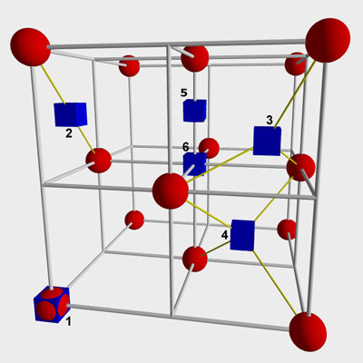
|
To produce a Waterman Polyhedron from a CCP lattice of atoms:
- Define a large sphere inside the lattice. Retain the cluster of atoms whose centers are inside your large sphere (or on its surface). Throw away atoms whose centers are outside your sphere. Hopefully your sphere was big enough to enclose at least 4 atoms that don't all lie in the same plane.
- Form the smallest convex polyhedron that contains the center points of the enclosed atoms.
Traditionally, Waterman Polyhedra are generated with the large sphere centered on one of the atoms. But there's no reason to ignore other possible "origins". Other "origin" choices yield different series of polyhedra, having differing symmetry properties. This applet is able to generate polyhedra from 7 different origins.
This applet's Sequence Slider controls the size of the large sphere, and the applet's Origin Choice controls the origin.
Warning -- don't get confused -- there are two different spheres mentioned on this web page. The "large sphere" mentioned in this section encloses a cluster of atoms. But discussions of the Cubic Close Packing (CCP) refer to the packing of spheres. In that case, the spheres are the individual atoms.
The "Origin" Choice
The available origins correspond to the numbered blue cubes in the diagram (above).They're listed here (and in the Choice Box) in order of my preference.
- 1=Atom Center:
This is the traditional origin from which Waterman Polyhedra are generated. The polyhedra in this series have the same symmetry properties as a cube. The first polyhedron (Seq=1) is a cuboctahedron whose vertices correspond to the 12 atoms that are equidistant from the origin (the central atom). - 6=Octahedral Void Center Between 6 Atoms:
The polyhedra in this series have the same symmetry properties as a cube. The first polyhedron (Seq=1) is an ocahedron whose vertices correspond to the 6 atoms that are equidistant from the origin. - 4=Tetrahedron Void Center Between 4 Atoms:
The polyhedra in this series have the same symmetry properties as a tetrahedron. The first polyhedron (Seq=1) is a tetrahedron whose vertices correspond to the 4 atoms that are equidistant from the origin. - 2=Touch Point Between 2 Atoms:
The polyhedra in this series have the symmetry of a flat rectangle whose top and bottom faces are the same (so turning it over is a symmetry). We call this origin the "Touch Point" because this is where two atoms would touch each other if they were expanded. - 5=5 Atoms:
This origin is halfway between an atom and an Octahedral Void Center. The polyhedra in this series have the symmetry of a flat rectangle whose top and bottom faces are different (so turning it over is not a symmetry). The first polyhedron (Seq=1) is a square pyramid whose vertices correspond to the 5 atoms that are closest to the origin - 3=Void Center Between 3 Atoms:
The polyhedra in this series have the symmetry of a flat triangle whose top and bottom faces are different (so turning it over is not a symmetry). The first polyhedron (Seq=1) is the same tetrahedron that's generated by origin 4, except it's shifted off-center. - 3*=Void Center Between 3 Lattice Voids:
This origin is designated "3 star". It's not shown in the diagram, but the point that's 1 unit directly below origin 3 could be labelled 3*. It's equidistant from 3 unoccupied lattice intersections in the same way that origin 3 is equidistant from 3 occupied lattice intersections. Origin 3* has the same symmetry as origin 3. If all the occupied lattice intersections became unoccupied and vice versa, origin 3 would become origin 3*. The relationship between 3 and 3* is the same as the relationship between 1 and 6.
Historical Notes:
I asked Steve Waterman about the history of these polyhedra.Here's what he told me (slightly paraphrased):
|
"In 1988, I wanted to make a Risk map that I could use as a globe, that is, I wanted to use it to fly over the poles, for example.
Unable to find a Dymaxion Map at the local University (due to mis-filing), I ended up trying to make a Dymaxion map
from an inferior 8 1/2 x 11 inch version I had.
If I had found the Map, I would not have done ANY of my sphere packing, cartographic or subsequent physics work/theories.
That got me to experimenting with other things... like a net of hexes to cover a globe. I made some versions, and then thought about the packing of spheres. I saw in a book , (do not have the title) where Fuller's VE had 12 spheres surrounding 1 sphere and wondered about how to extend this format in comparison to his method of inclusion. So, I tried to work out the math involved. Built planes with a sphere in the center, worked out distance formulas within the plane. Then got the no sphere at center plane distancing,... and its formula. Then, I got a formula for the distance between planes. That all took about two years to do.... to finally realize that all that math meant distances were confined to integer roots of a radial sweep. This I followed up, by doing all this again, but not as a sphere with 6 spheres around it, for the ABC layering... but as a corresponding system the ABA formulas... and have the output results match in both cases from a sphere-center origin. I had a big chart, where I had all the sphere counts per distance per z level up to root 1000 for the ABC, and went to just root 100 for the ABA, seeing that the sphere count coincided. I stopped the ABA, and decided that it should now be computerized, and that all we needed was the integer and there was a unique polyhedron that related to that integer. My Eureka moment here came when I became aware that I could turn the math into polyhedra. Years pass, and Kirby Urner in 1995(?) uses Python to make the convex hull from the point set as determined only by that radial sweep parameter. Then skip ahead a few more years and Paul Bourke 2002(?) writes his code in POV-Ray that uses root 2 diameter spheres, giving us all integer coordinates." |
I also got a note from Kirby Urner:
| "I collaborated with Steve a long time ago generating said polys (and suggesting they be called Watermans) using Python + POV-Ray." |
Related Web Pages:
- Steve Waterman -- Discoverer of Waterman Polyhedra.
- Paul Bourke's Waterman Polyhedra Pages -- Explanations, graphics, monster polyhedra.
- Visualizing Waterman Polyhedra with MuPAD -- Nice article with graphics and explanations.
- Spheres and Polyhedra.
Acknowledgements:
This applet was suggested by Steve Waterman, discoverer and researcher of Waterman Polyhedra. Steve's correspondence guided and motivated the development of this applet.John Lloyd's open-source Robust 3D convex hull algorithm in Java is incorporated into the applet. The fantastic speed and ease-of-use of John's routines was the final deciding factor in my choice to write this applet.
Paul Bourke's site has graphics, algorithms and explanations which were very helpful during the development of this applet. His POV-Ray code was the starting point for my Waterman-generation algorithm.
The 3D renderer is of my own invention. The symmetric and chiral coloring algorithms are my own.
Version Notes:
- Version 1.1
May 15, 2005- Initial Release
- Version 1.2
March 31, 2009- Increased Range of Sequence Slider:
At the request of Steve Waterman, I increased the sequence limit from 2000 to 3000. - Colors:
The colors are probably more vivid due to some recent tinkering with the color generator.
- Increased Range of Sequence Slider:
Polyhedron Statistics:
The applet can print some statistics for each polyhedron. Here's an example:================================================== Seq=1132 Origin 1 Radius=sqrt(2N) N=1233 #atoms...: 256613 #vertices: 1392 #faces...: 1634 #edges...: 3024 #colors..: symmetric=44, chiral=70 radius...: 49.658836 area.....: 30851.78 (0.9955825 of enclosing sphere) volume...: 508470.66 (0.99126023 of enclosing sphere) volume divided by #atoms: 1.9989392 convex hull calculation: #input points: 15514 time: 250 milliseconds max of the calculateHorizon "cnt" variable: 12 ==================================================
The statistics are printed to your Java console, so the first step is to find the Java console. Check your browser documentation, or if you're using the Java Plugin, check the Plugin documentation.
To cause the applet to start printing statistics, you need to perform a "secret action":
Click the mouse on the polyhedron, and without releasing the mouse button, type 4 letters:
s h o w
(This requires 2 hands.)
As soon as you type the "w", the applet will begin printing statistics (and you can release the mouse button).
#atoms is the total number of atom centers within the enclosing sphere of the specified radius.
#input points is a count of the surface atoms that were input to the convex hull routine.
Distances are specified in units of the lattice distance (the distance between lattice intersections in the diagram).
<Dogfeathers Home Page> <Mark's Home Page> <Mark's Java Stuff>
Email: Mark Newbold
This page URL: http://dogfeathers.com/java/ccppoly.html
Copyright 2005 by Mark Newbold. All rights reserved.
![]()
![]()
![]()
![]()
![]()
![]()